Gradient Attacks

Welcome to the second post in the AI Village’s adversarial machine learning series. This one will cover the greedy fast methods that are most commonly used. We will explain what greedy means and why certain choices were made that may not be obvious to newcomers. This is meant as a read-a-long with the papers, we will not be going into a lot of detail but we will focus on the explaining the tricky minutia so that you can understand these papers more easily.

We have made a library that demonstrates these attacks. There’s a useful template class in there that we’ll be extending BaseAttack. It has methods for testing the effectiveness of the attack and visualization to make debugging these attacks easier. However you still need to implement the attacks yourself. All the images and results in this post come from this script.

In the rest of that repo you can also find target models and datasets to play around with. We’re using the ResNet CIFAR10 model for these demonstrations, but if you don’t have GPU handy you can use the MNIST MLP model. If you’re in a CTF you will be supplied with those models and an associated pickle so that we’re all on the same page.

The Problem and Optimization

Recall the definition:

Definition: Let \(f: \mathbb{R}^N \to \{L_1,L_2, \dots L_n\}\) be a function whose range is a discrete set of labels, let \(x\) such that \(f(x) = L_i\), and let \(\hat{x}\) such that \(\lVert x-\hat{x} \rVert_p < \epsilon\) such that \(f(\hat{x}) = L_j\) and \(i \neq j\). Then \(\hat{x}\) is an adversarial example with threshold \(\epsilon\).

We want to find the closest adversarial examples, so what we are trying to do is come up with a perturbation \(h = x - \hat{x}\) such that we change the result of the classifier. Since we’re trying to show that these are dumb machines, this perturbation should be the “shortest” or least noticeable. The classic distance is the \(L_2\) norm, but we can also pick two other norms that often come up in machine learning, \(L\_1\) and \(L\_\infty\).

A Quick Review of Stochastic Gradient Descent

Our classifier usually uses a one hot encoding for the labels of the data. So, an element of our \(i\)th class should be mapped by our classifier to a vector that has a 1 in the \(i\)th slot and a \(0\)s everywhere else. It doesn’t do this perfectly so we use a loss function to gauge the error between the desired one hot output and the true label. What is important here about the loss function is that it maps to the reals, \(\mathbb{R}\). So, with our training data, \((x,y)\) and our neural network we can get the loss of the network at that input point with that label, \(L(N(x),y)\), usually written as \(J(x,y)\). You should think of this as a height map with low points where the model is correct and high points where the model is wrong.

Normally we descend the gradient over the parameters that the network (or any other model that is differentiable) uses, \(\theta\). The variable \(\theta\) is all parameters in the model, the matrix and bias in a fully connected layer, the convolutional filters, lumped together. These are suppressed in the notation \(N(x)\) and \(J(x,y)\) like class attributes, but we can make it functorial and explicit by writing \(N(x,\theta)\) and \(J(x,y,\theta)\). When we train a network we actually travel over the surface defined by \(J(x,y,\theta)\) with respect to \(\theta\).

High error is bad and the direction to increase the error the fastest at \((x\_i,y\_i)\) is the gradient, \(\nabla\_{\theta}J(x\_i,y\_i,\theta)\). Therefore, we go the opposite direction by a step, \(\theta\_{i+1}=\theta\_{i}-\epsilon \nabla\_{\theta} J(x\_i,y\_i,\theta\_{i}),\)

where the \(\epsilon\) is a small value we chose. Do this in a randomized loop over all your data several times and you’ve got Stochiastic Gradient Descent. Think of this as rolling down a very complex hill in \(\theta \in \mathbb{R}^D\) where the dimension, \(D\), can be in the millions.

Simplest Attack

Since we’re attacking models instead of training them, we consider \(\theta\) a fixed parameter. We want to change \(y\) with respect to \(x\). So what direction does \(\nabla_x J(x,y)\) point in? It points up the hill of error, so to move the output \(N(x)\) fastest away from the correct value in \(x\) space we ascend the gradient.

If we want to move in the direction that will increase the loss the most by a step of \(\epsilon\), we can do this: \(\hat{x} = x + \epsilon \nabla_x J(x,y)\)

class GradientAttack(BaseAttack):
	def __init__(self, model, loss, epsilon):
		super(GradientAttack, self).__init__()
		self.model = model
		self.loss = loss
		self.epsilon = epsilon

	def forward(x,y_true):
		# Give x a gradient buffer
		x_adv = x.requires_grad_()

		# Build the loss function at J(x,y)
		y = self.model.forward(x_adv)
		J = self.loss(y,y_true)

		# Ensure that the x gradient buffer is 0
		if x_adv.grad is not None:
			x_adv.grad.data.fill_(0)

		# Compute the gradient 
		x_grad = torch.autograd.grad(J, x_adv)[0]

		# Create the adversarial example and ensure 
		x_adv = x_adv + self.epsilon*x_grad

		# Clip the results to ensure we still have a picture
		# This CIFAR dataset ranges from -1 to 1.
		x_adv = torch.clamp(x_adv, -1, 1)

		return x_adv

Lets step through this line by line. First we initialize the attack with the parameters we want to use. BaseAttack wants our attack to be implemented in the forward method of torch.nn.Modules, so we do that. We are going to be supplying raw images to this function, so we need to make pytorch allow us to take the gradient of \(J\) with respect to \(x\).

Since this is an untargeted attack we primarily care about if the attack changed the label that the model assigns to that sample. In the gradient method’s case we have the following results:

The three images are, the base classes, the modified classes, and 10 times the difference. In the center we show red for an unsuccessful attack and green for a successful one.

Our attack is quite a failure. Clearly something needs to be fixed. One thing we can do is to iterate our attack until it successfully confounds the classifier, you can try this by adding a loop and making this a simple gradient descent. However this will result in perhaps hundreds of calls to the perhaps computationally intense model, as well as equally many calls to the automatic differentiation package.

Normalized Gradient Attack

One of things to note is that the difference in the gradient method is really faint. This is because at the bottom of the neural network the gradient may be very small. The gradients we see on these samples range in \(L_2\) length from \(0.003\) to \(0.000002\). To put this in context the average distance between two points in the image space (a 3072 dimensional hypercube) is somewhere between 18 and 40, and not 0.333 like a line. So, we’re actually moving an absolutely tiny amount. To compensate for this, lets normalize our step, i.e. take the same length step every time: \(\hat{x} = x + \epsilon \frac{\nabla_x J(x,y)}{\lVert \nabla_x J(x,y) \rVert_2}\)

To do this change the line where we make the adversarial example to:

x_norm = x_grad.view(x_grad.size()[0], -1)
x_norm = F.normalize(x_norm)
x_norm = x_norm.view(x_grad.size())

x_adv = x_adv + self.epsilon*x_norm

Lets see how well this works:

This clearly enjoys a much greater success rate! We move much further. We also move exactly \(\epsilon\) away from the original, so in competitions where the challenge is to minimize the distance between the normal and adversarial points, we can directly tune this parameter. However it is also the only thing we can tune, so there may be a better way.

Fast Gradient Sign Method

The final modification of the gradient method is inspired by the \(L_\infty\) norm. This is very closely related to image stenography where you can manipulate the last bit of the RGB values per pixel without a human noticing. This is also the usual introduction, it’s more successful than the normalized gradient method, even faster to compute, and easier to code.

Looking back at the normalized gradient method, we can think of it as moving as far as possible in the “best” direction. We’ve taken a greedy guess at the best direction with the gradient, there might be a better direction that’s not the same as the gradient. We then take the biggest step possible, while staying inside the sphere of radius \(\epsilon\). This process happens in a high dimensional sphere, but it’s not too different from the low dimensional one.

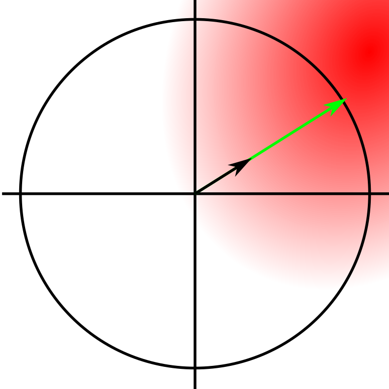
The gradient in this image is the black arrow, the adversarial step is the green one, and the quantity of red is the height of the loss function. We can see that we’ve stepped right to the border. However there’s darker, higher loss areas just outside of the circle.

For \(L_\infty\) we can move further, we are constrained by a high dimensional cube with side lengths \(2\epsilon\) instead of a sphere of radius \(\epsilon\). The corners of the cube are much further out than the surface of the sphere. To see this we can look at the same situation as above, but with a square instead of a circle.

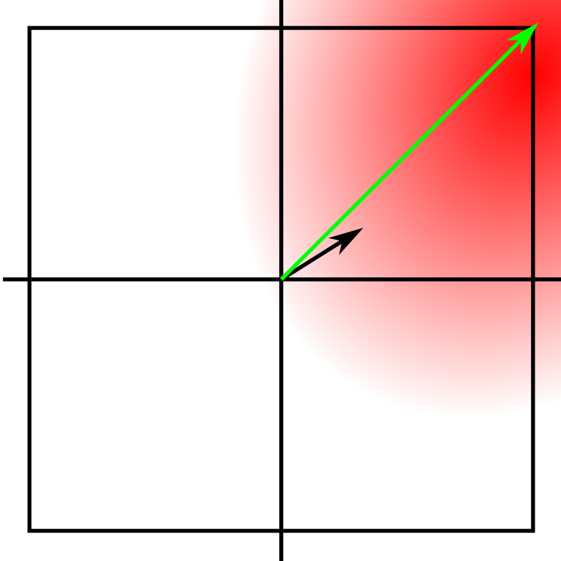
Our best guess is to move to the corners. The space is small and we’re probably on a close to linear slope, so it is a good bet. To do this we don’t normalize the gradient we take the sign of the gradient. \(\hat{x} = x + \epsilon \text{sign}(\nabla_x J(x,y))\) This is accomplished by switching out the creation line in the gradient attack with the following:

x_adv = x + self.epsilon*x_grad.sign_()

To see this attack, with the same epsilons as before:

Clearly the most effective so far. However, you can see that we really should stick to low \(\epsilon\)s else it overwhelms the image.

Improvements

We can significantly improve these attacks if we were less greedy and took our time. If we took smaller steps, and constrained our movement we could do get similar success rates but remain bit closer to our original image. The next post will be a little shorter and cover these iterative methods.

• 2023 5
• 2022 7
• 2018 3